Below you can find some instructions on how to install and use ssNake, for processing and analyzing NMR data.

Installation

Windows - Standalone

You can obtain an executable ssNake v1.4 installer through this link or check for the latest version here. The installation is straightforward and will leave you with an executable to directly launch the software.

Linux / Python source code

In order to run ssNake on Linux or on any other operating system with a present Python 3 installation, you can directly download its source code or use git to clone it into a new directory:

mkdir ssNakeDir #This line is optional
git clone https://github.com/smeerten/ssnake.git ssNakeDir

(or simply)

git clone https://github.com/smeerten/ssnake.git

After downloading you can simply execute ssNake.py with Python inside the “src” directory inside the installation folder:

python3 ssNakeDir/src/ssnake.py

Processing data

Once ssNake’s GUI is loaded, you can open a new dataset via File --> Open which will either display an FID (like in my case) or a spectrum, depending on whether your data was already processed before or not. Typically, data imported from Bruker’s Topspin will show up as spectrum. In this example I loaded a $^{29}$Si MAS NMR experiment on a lithium disilicate glass measured on a Varian machine:

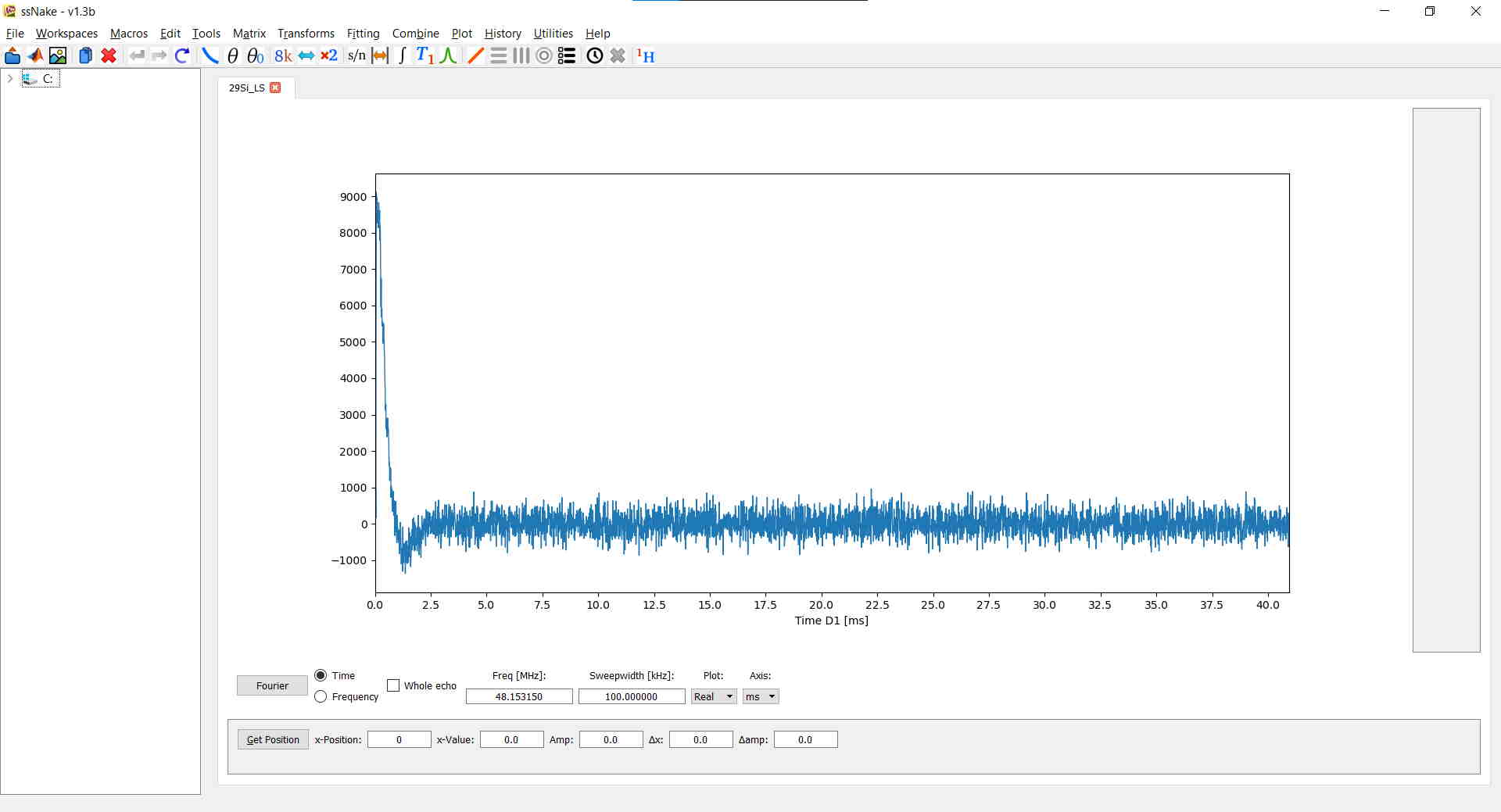
The most common processing functionalities are found in the Tools and Matrix tabs. For the current example I truncated the FID after 1024 points using Matrix --> Sizing and after applied the changes by clicking on “ok”. Next, I performed a zero-filling up to 2048 points. The resulting FID looks like this:

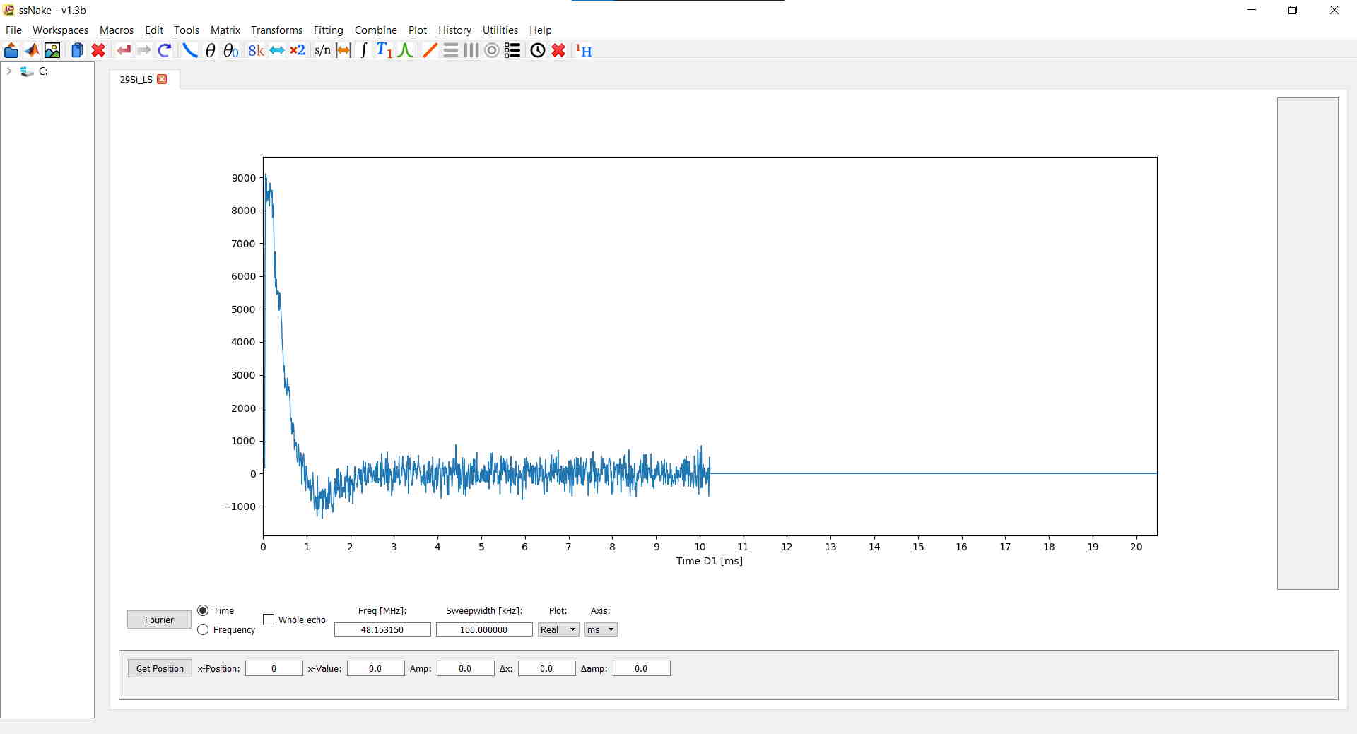
A window function can be applied via Tools --> Apodize. In the current example I applied a Gaussian window function with roughly 100 Hz of width. Note how the window function is displayed in green and the raw FID remains as a gray shade:

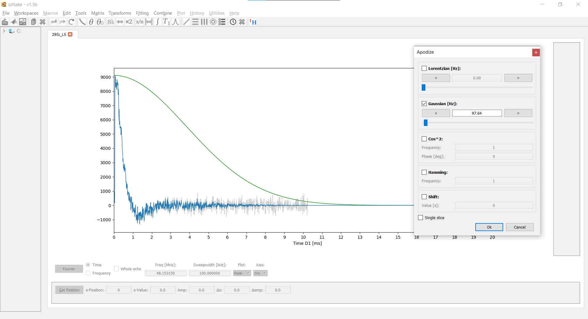
Lastly, I shifted the FID six points to the left via Matrix --> Shift Data:

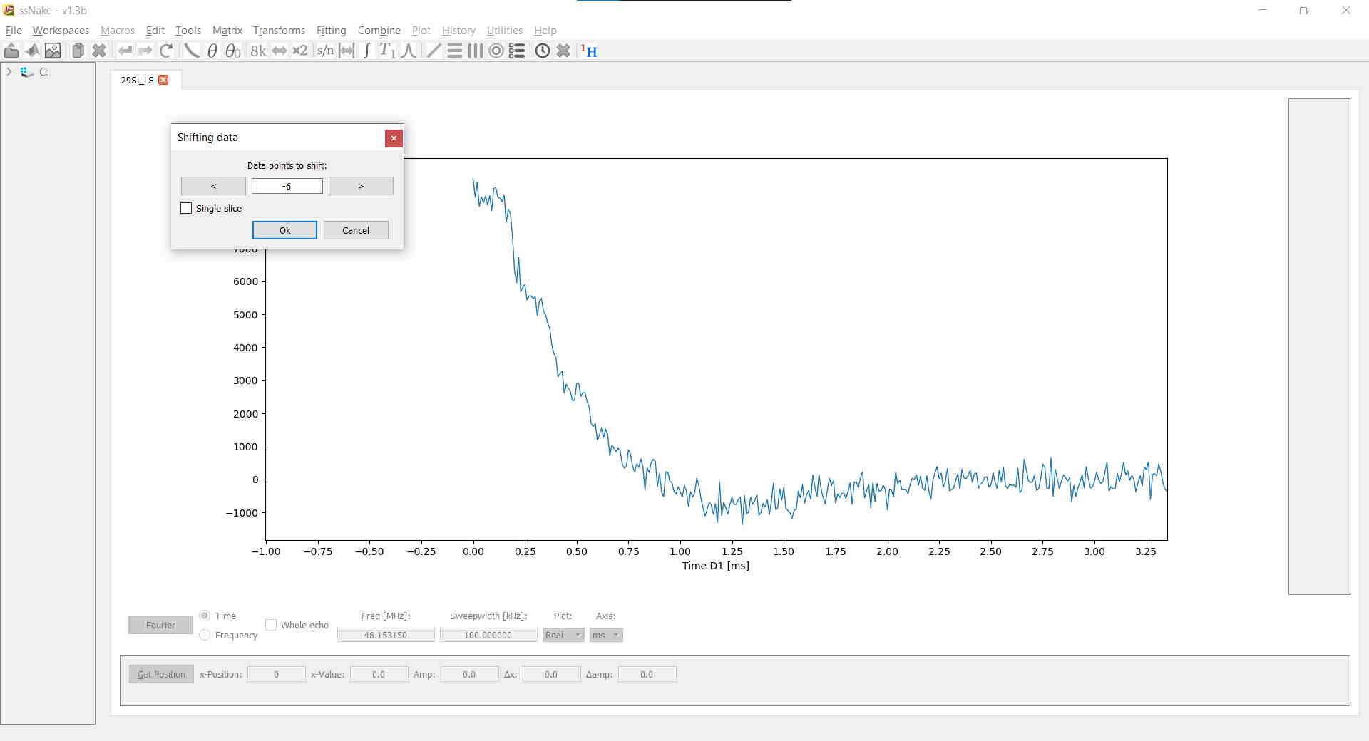
By the way, you can zoom-in and -out of your data by dragging a box with your left-mouse button, drag your data around with the right-mouse button, scale your data with the mouse-wheel, and - perhaps most importantly - reset to the default view by double-right clicking.

Once we are all set we can finally do a Fourier-Transform of the FID by clicking on the button in the bottom-left corner of the main window labeled ‘Fourier’ or, aLternatively, use the shortcut Ctrl + F, or do it via Transforms --> Fourier Transform. For my data this results in the following spectrum:

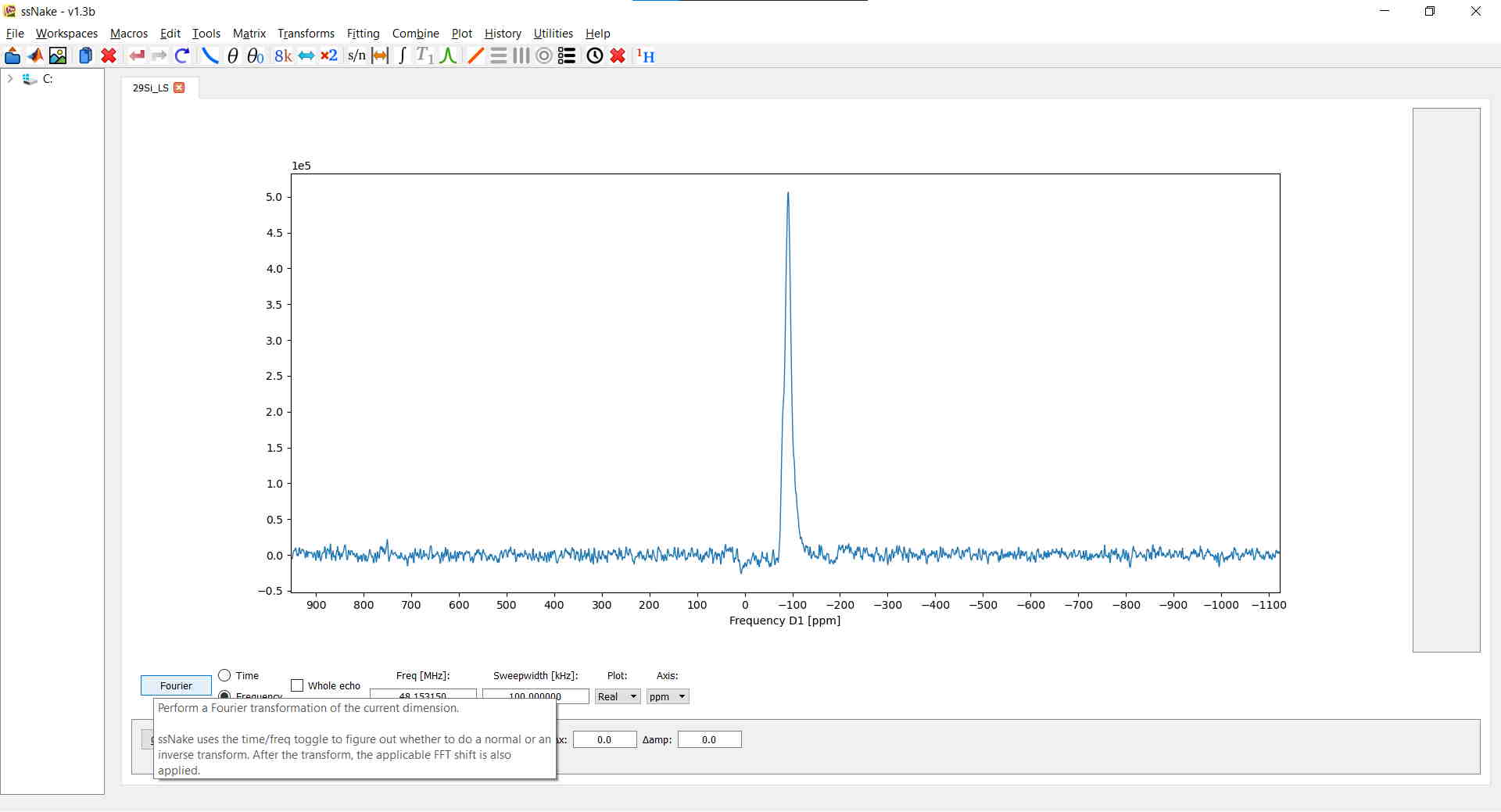
Before continuing you might want to change the abscissa label to ppm instead of Hz. This can be done in the Axis tab below the spectrum:

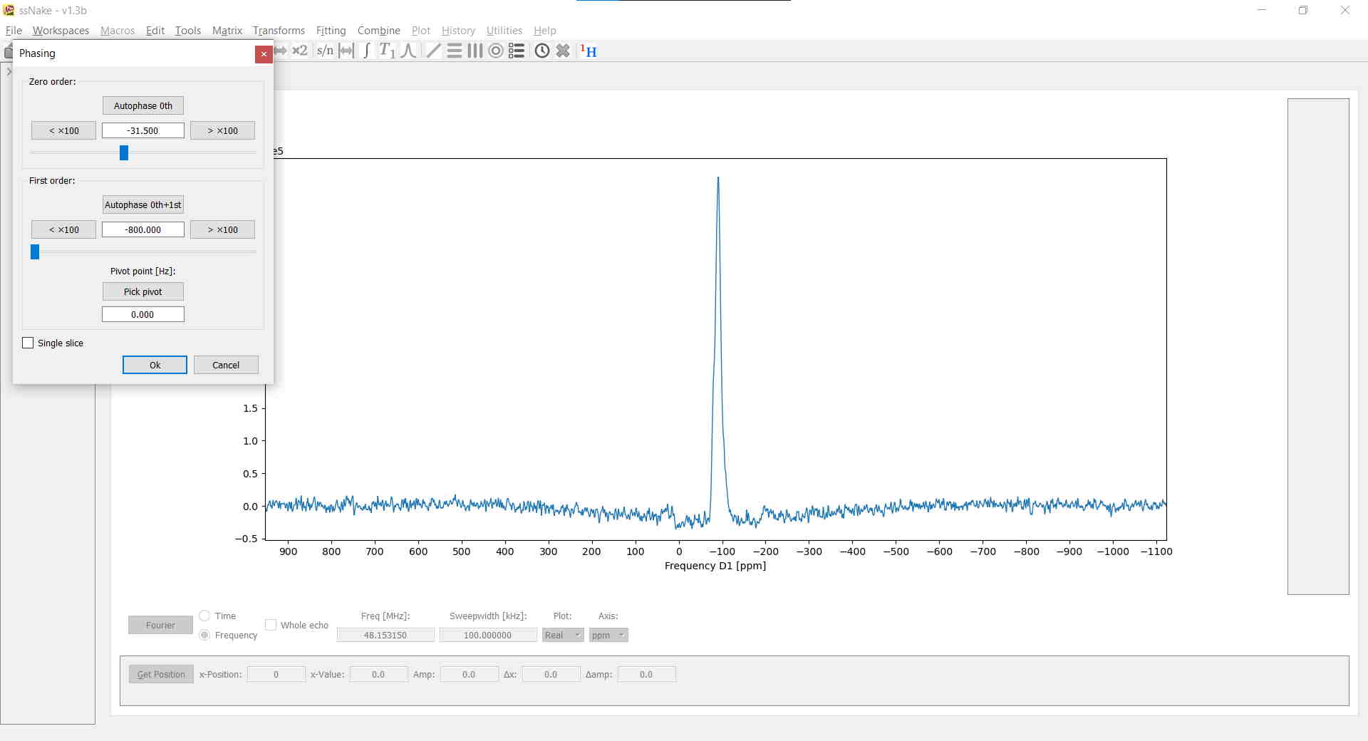
Now it’s time to correct the phase. Tools --> Phasing -> Phase will take you to the interactive phase correction window in which you can apply zeroth- and first-order phase correction by clicking on the respective arrow buttons. Note that by holding down Ctrl or Shift you can apply a 10x or 100x multiplier to the applied amount on each click. Here, I applied enough first-order correction to get the barely visible spinning-sidebands facing up and then adjusted the zero-order correction accordingly:

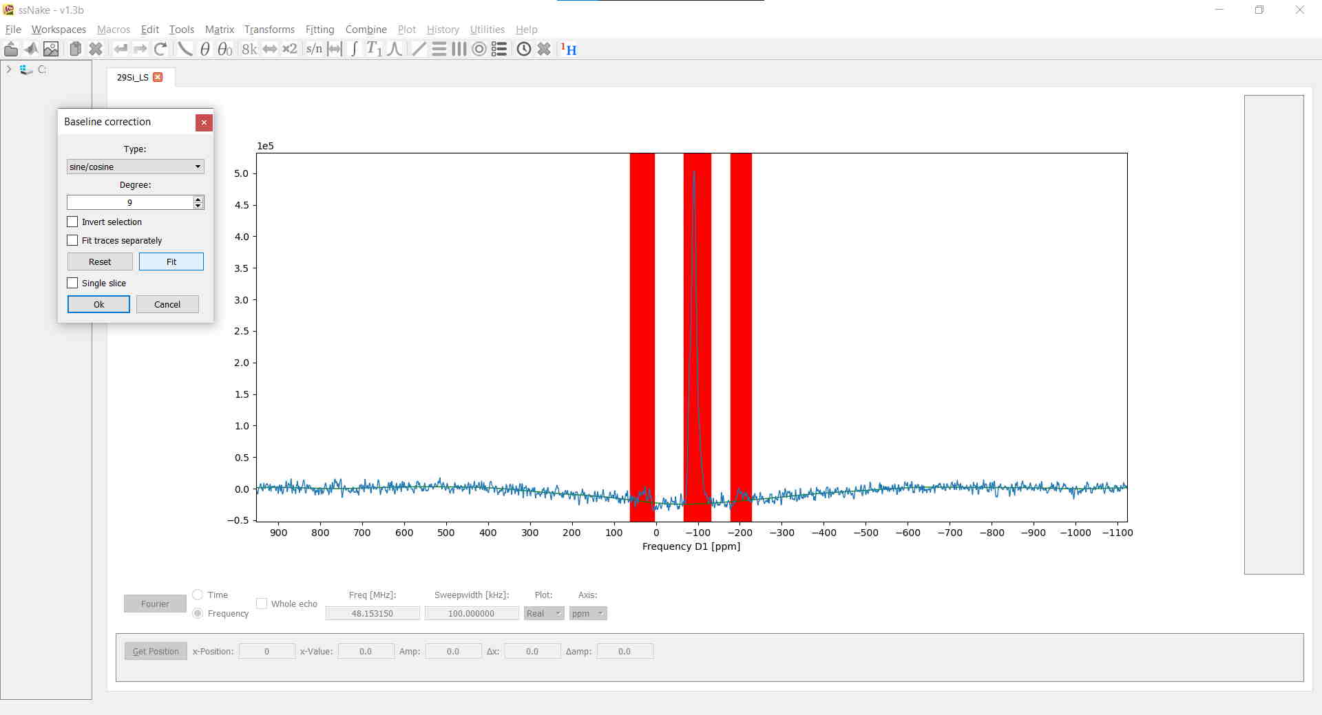
At this point the spectrum looks already pretty decent. A baseline correction, however, will surely help with lineshape deconvolution later on. In ssNake, baseline corrections, accessible via Tools --> Baseline Correction, are implemented in a rather clever way. Instead of spline fitting, often encountered in other software, the baseline will be fitted using a polynomial or sine/cosine function. Conveniently you get to select which parts of the spectrum are to be ignored, namely all NMR signals. The latter is done by left-clicking once to mark the onset of an NMR signal and left-clicking a second time to span a region which is then marked in red. Lastly, the degree of the fitting function is defined - best chosen by some trial-and-error - and clicking on Fit. The result may then look similar to this:

Now you are basically done. In my case, I find it convenient to additionally normalize my data with respect to the signal maximum which makes fitting the data easier afterwards:

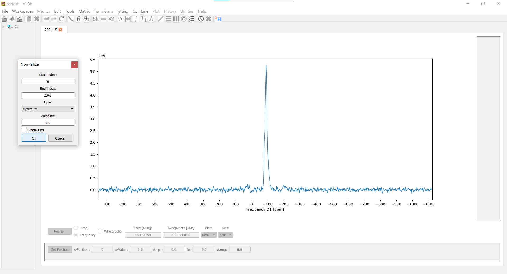
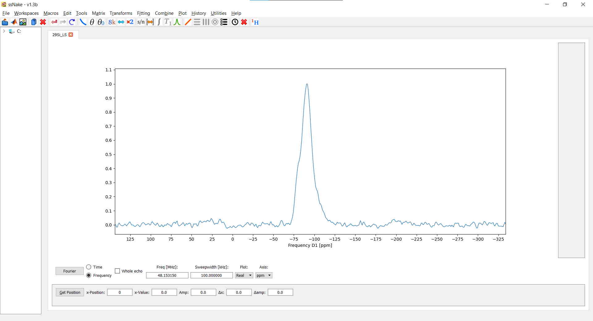
The final result of the $^{29}$Si MAS NMR spectrum of a vitreous lithium disilicate sample then looks like this: